Measuring Residential Segregation

Introduction

In this lab, we’ll explore some of the common measures of residential segregation and apply them at the city and regional levels.

In our last lab, we got a basic idea of the racial distribution for census tracts. Now we can start to think about summary measures of the extent to which these groups are segregated within the region. We will use census tracts as a unit of analysis to help us describe county-level racial segregation.

Most measures of residential segregation are set up to summarize the level of heterogeneity (or homogeneity) observed between neighborhoods to a city or regional scale to produce a summary measure that then tells us how even populations are distributed at the neighborhood level.

There are also some measures that focus more on segregation at a neighborhood level. In this lab, we’ll focus on those measures that summarize characteristics to more aggregate levels such as cities or regions.

Goals

Gain exposure to common measures of residential segregation.
Learn how to apply simple measures within R / RStudio.

Core Concepts

R and Rstudio

[concepts here]

Let’s get going…

Github Lab Repository

Follow this link to accept the lab Github Classroom assignment repository.

Setup

Let’s start as usual by loading the packages that we’ll need for our work.

Code

library(gt)
library(tigris)
library(tidycensus)
library(tidyverse)
library(sf)

For the purposes of our example, we’ll continue examining racial segregation in New York City - an extension of our previous lab example. Let’s start by downloading and preparing data on race for New York City.

Get Tract Boundaries

Let’s download 2020 census tract boundaries for New York City’s five Boroughs. While we’re at it, we’ll clean them up a little bit as we did in our last lab.

New York City Boroughs
FIPS Code	County Name	Borough Name
36047	Kings County	Brooklyn
36005	Bronx County	Bronx
36081	Queens County	Queens
36085	Richmond County	Staten Island
36061	New York County	Manhattan

Code

nyc_trt <- tracts(state = "NY", county = c("005", "047", "061", "081", "085"), year = 2020) |> 
  st_transform(26918) |> 
  filter(ALAND != 0) |> 
  erase_water(area_threshold = .9, year = 2020)


  |                                                                            
  |                                                                      |   0%
  |                                                                            
  |                                                                      |   1%
  |                                                                            
  |=                                                                     |   1%
  |                                                                            
  |=                                                                     |   2%
  |                                                                            
  |==                                                                    |   2%
  |                                                                            
  |==                                                                    |   3%
  |                                                                            
  |===                                                                   |   4%
  |                                                                            
  |===                                                                   |   5%
  |                                                                            
  |====                                                                  |   5%
  |                                                                            
  |====                                                                  |   6%
  |                                                                            
  |=====                                                                 |   7%
  |                                                                            
  |=====                                                                 |   8%
  |                                                                            
  |======                                                                |   8%
  |                                                                            
  |======                                                                |   9%
  |                                                                            
  |=======                                                               |  10%
  |                                                                            
  |========                                                              |  11%
  |                                                                            
  |========                                                              |  12%
  |                                                                            
  |=========                                                             |  12%
  |                                                                            
  |=========                                                             |  13%
  |                                                                            
  |===========                                                           |  16%
  |                                                                            
  |============                                                          |  16%
  |                                                                            
  |============                                                          |  18%
  |                                                                            
  |=============                                                         |  19%
  |                                                                            
  |=================                                                     |  24%
  |                                                                            
  |====================                                                  |  29%
  |                                                                            
  |=======================                                               |  33%
  |                                                                            
  |========================                                              |  34%
  |                                                                            
  |========================                                              |  35%
  |                                                                            
  |=========================                                             |  35%
  |                                                                            
  |=========================                                             |  36%
  |                                                                            
  |==========================                                            |  37%
  |                                                                            
  |===========================                                           |  39%
  |                                                                            
  |============================                                          |  40%
  |                                                                            
  |=============================                                         |  41%
  |                                                                            
  |=============================                                         |  42%
  |                                                                            
  |==============================                                        |  42%
  |                                                                            
  |==============================                                        |  43%
  |                                                                            
  |===============================                                       |  44%
  |                                                                            
  |===============================                                       |  45%
  |                                                                            
  |================================                                      |  45%
  |                                                                            
  |==================================                                    |  48%
  |                                                                            
  |==================================                                    |  49%
  |                                                                            
  |===================================                                   |  50%
  |                                                                            
  |====================================                                  |  51%
  |                                                                            
  |====================================                                  |  52%
  |                                                                            
  |======================================                                |  54%
  |                                                                            
  |======================================                                |  55%
  |                                                                            
  |=======================================                               |  56%
  |                                                                            
  |========================================                              |  56%
  |                                                                            
  |========================================                              |  57%
  |                                                                            
  |========================================                              |  58%
  |                                                                            
  |=========================================                             |  58%
  |                                                                            
  |=========================================                             |  59%
  |                                                                            
  |==========================================                            |  60%
  |                                                                            
  |==========================================                            |  61%
  |                                                                            
  |===========================================                           |  61%
  |                                                                            
  |===========================================                           |  62%
  |                                                                            
  |============================================                          |  62%
  |                                                                            
  |============================================                          |  63%
  |                                                                            
  |=============================================                         |  64%
  |                                                                            
  |=============================================                         |  65%
  |                                                                            
  |==============================================                        |  66%
  |                                                                            
  |===============================================                       |  67%
  |                                                                            
  |===============================================                       |  68%
  |                                                                            
  |================================================                      |  68%
  |                                                                            
  |================================================                      |  69%
  |                                                                            
  |=================================================                     |  70%
  |                                                                            
  |=================================================                     |  71%
  |                                                                            
  |==================================================                    |  71%
  |                                                                            
  |==================================================                    |  72%
  |                                                                            
  |===================================================                   |  73%
  |                                                                            
  |====================================================                  |  74%
  |                                                                            
  |====================================================                  |  75%
  |                                                                            
  |=====================================================                 |  75%
  |                                                                            
  |=====================================================                 |  76%
  |                                                                            
  |======================================================                |  77%
  |                                                                            
  |======================================================                |  78%
  |                                                                            
  |========================================================              |  80%
  |                                                                            
  |=========================================================             |  81%
  |                                                                            
  |=========================================================             |  82%
  |                                                                            
  |==========================================================            |  83%
  |                                                                            
  |===========================================================           |  84%
  |                                                                            
  |===========================================================           |  85%
  |                                                                            
  |============================================================          |  86%
  |                                                                            
  |=============================================================         |  86%
  |                                                                            
  |=============================================================         |  87%
  |                                                                            
  |=============================================================         |  88%
  |                                                                            
  |==============================================================        |  88%
  |                                                                            
  |==============================================================        |  89%
  |                                                                            
  |===============================================================       |  90%
  |                                                                            
  |===============================================================       |  91%
  |                                                                            
  |================================================================      |  91%
  |                                                                            
  |================================================================      |  92%
  |                                                                            
  |=================================================================     |  92%
  |                                                                            
  |=================================================================     |  93%
  |                                                                            
  |==================================================================    |  94%
  |                                                                            
  |==================================================================    |  95%
  |                                                                            
  |===================================================================   |  95%
  |                                                                            
  |===================================================================   |  96%
  |                                                                            
  |====================================================================  |  97%
  |                                                                            
  |====================================================================  |  98%
  |                                                                            
  |===================================================================== |  99%
  |                                                                            
  |======================================================================| 100%

As a reminder, the code above is accomplishing the following things:

Download tract-level census geometries as a simple features object for Kings, Bronx, Queens, Richmond, and New York Counties for the year 2020.
Transform these geometries to NAD 1983.
Remove those defined tract boundaries with no land area.
Erase the portion of tract boundaries that are water, focusing on the top 10 percent of largest defined water polygons, and using hydrography defined by the census in 2020.

Let’s use ggplot() to visualize so that we can confirm what we’ve downloaded is indeed New York City’s boroughs:

Code

ggplot()+
  geom_sf(data=nyc_trt)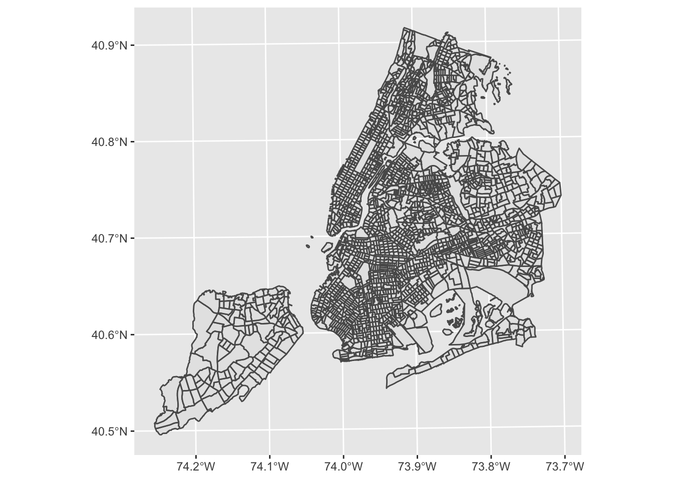

Get ACS Data

Next, we’ll download ACS data on race for New York City. We’ll focus on 2020 data from the 5-year ACS from Table B03002.

To keep things organized, let’s define the variables we want to download. Note that we’re defining variable names as well as values. To facilitate some of our later operations, let’s download these data in wide format rather than tidy format. In wide format, we’ll have one observation (row) for each census tract, with multiple columns containing estimates for each population subgroup and the total population.

Code

dl_vars <- c(
  White = "B03002_003",
  Black = "B03002_004",
  Native = "B03002_005",
  Asian = "B03002_006",
  HIPI = "B03002_007",
  Hispanic = "B03002_012",
  Poptot = "B03002_001"
)

# Our tidycensus download call:

nyc_race <- get_acs(
  geography = "tract",
  state = "NY",
  county = c("Bronx", "Kings", "New York", "Queens", "Richmond"),
  variables = dl_vars,
  year = 2020,
  output = "wide"
) 

nyc_race |> 
  slice_head(n = 5) |> 
  gt()

GEOID	NAME	WhiteE	WhiteM	BlackE	BlackM	NativeM	AsianE	AsianM	HIPIM	HispanicE	HispanicM	PoptotE	PoptotM
36047009202	Census Tract 92.02, Kings County, New York	328	96	162	129	12	1037	293	12	1904	630	3453	653
36047009401	Census Tract 94.01, Kings County, New York	132	72	173	245	12	1582	389	12	406	283	2293	380
36047009402	Census Tract 94.02, Kings County, New York	377	198	38	57	12	1903	586	12	271	213	2746	553
36047009600	Census Tract 96, Kings County, New York	1035	313	78	60	17	1993	519	17	2629	629	5858	710
36047009800	Census Tract 98, Kings County, New York	218	83	162	160	17	2306	504	17	3275	740	6021	798

Note that tidycensus downloads the data, and labels each column with the label we have defined (with E and M denoting estimates and margins of error).

While we’re at it, let’s separate our tract name label into separate tract, county, and state values.

Code

nyc_race <- nyc_race |> 
  separate(NAME, into = c("Tract", "County", "State"), sep = ", ")

Note the use of sep = ", " includes the space after the comma so we don’t have an extra space in our resulting county and state variables.

Create County Summaries

Before we further manipulate our data, let’s aggregate the data we have to form county population summaries. Because our tract data is hierarchical, we can sum up our population estimates from tracts to counties to produce county population totals. While we’re at it, we’ll also use the county FIPS codes to create a Borough identifier (we could also add county labels back as well).

Code

nyc_race_co <-
  nyc_race |> 
  group_by(STCO = substr(GEOID, 0, 5)) |> 
  summarise(
    co_WhiteE = sum(WhiteE, na.rm = TRUE),
    co_WhiteM = moe_sum(WhiteM, WhiteE),
    co_BlackE = sum(BlackE, na.rm = TRUE),
    co_BlackM = moe_sum(BlackM, BlackE),
    co_NativeE = sum(NativeE, na.rm = TRUE),
    co_NativeM = moe_sum(NativeM, NativeE),
    co_AsianE = sum(AsianE, na.rm = TRUE),
    co_AsianM = moe_sum(AsianM, AsianE),
    co_HIPIE = sum(HIPIE, na.rm = TRUE),
    co_HIPIM = moe_sum(HIPIM, HIPIE),
    co_HispanicE = sum(HispanicE, na.rm = TRUE),
    co_HispanicM = moe_sum(HispanicM, HispanicE),
    co_PoptotE = sum(PoptotE, na.rm = TRUE),
    co_PoptotM = moe_sum(PoptotM, PoptotE),
  ) |> 
  mutate(Borough =
    case_when(
      STCO == "36005" ~ "Bronx",
      STCO == "36047" ~ "Brooklyn",
      STCO == "36061" ~ "Manhattan",
      STCO == "36081" ~ "Queens",
      STCO == "36085" ~ "Staten Island")
  )

Let’s walk through this:

We are going to use group_by() to aggregate our tract-level data to counties. In this case, we are pulling out the first five digits from the combined state-county-tract FIPS code (substr(GEOID, 0, 5)) using the substr() command from the stringr package. This allows us to create a combined state and county FIPS code (the state is the first two digits - 36 in the case of New York - and the county is the next three digits).
We use summarise() to create summary values for counties. We use sum() on our population estimates to sum up populations for tracts into county totals. We use moe_sum() from the tidycensus() package to properly aggregate margins of error accounting for the size of the population estimate being aggregated. The census provides documentation on what’s implemented in tidycensus. We denote that these are county estimates by including co_ as a prefix - you’ll see why later.
We use case_when() construct borough labels from our combined state and county FIPS codes.

As a result, we have a table containing county populations and margins of error for the boroughs of New York City:

STCO	co_WhiteE	co_WhiteM	co_BlackE	co_BlackM	co_NativeE	co_NativeM	co_AsianE	co_AsianM	co_HIPIE	co_HIPIM	co_HispanicE	co_HispanicM	co_PoptotE	co_PoptotM	Borough
36005	128,717	3,742	411,293	8,800	2,882	727	53,498	3,097	374	198	799,765	12,002	1,427,056	14,216	Bronx
36047	938,573	10,493	754,576	10,307	3,053	638	304,420	6,367	1,009	480	486,272	9,181	2,576,771	17,237	Brooklyn
36061	763,202	11,503	199,377	6,238	1,960	581	196,097	6,049	430	237	418,442	9,769	1,629,153	16,500	Manhattan
36081	559,778	8,090	385,868	7,374	5,561	948	584,214	9,369	832	271	631,657	10,976	2,270,976	16,687	Queens
36085	286,462	6,247	43,941	2,970	515	243	47,194	2,905	55	127	87,733	4,193	475,596	7,858	Staten Island

Let’s create a more polished table showing the population by race for each NYC Borough:

Code

nyc_race_co |> 
  mutate(other = co_NativeE+co_HIPIE) |> 
  select(Borough, co_WhiteE, co_BlackE, co_AsianE, co_HispanicE, other, co_PoptotE) |> 
  gt() |> 
  fmt_number(2:7, decimals = 0) |> 
  cols_label(
    co_WhiteE = "White",
    co_BlackE = "Black",
    co_AsianE = "Asian",
    co_HispanicE = "Hispanic",
    other = "Other",
    co_PoptotE = "Total"
  ) |> 
  summary_rows(
    columns = 2:7, 
    fns = list(Total = ~sum(.)),
    formatter = fmt_number,
    decimals = 0)

	Borough	White	Black	Asian	Hispanic	Other	Total
	Bronx	128,717	411,293	53,498	799,765	3,256	1,427,056
	Brooklyn	938,573	754,576	304,420	486,272	4,062	2,576,771
	Manhattan	763,202	199,377	196,097	418,442	2,390	1,629,153
	Queens	559,778	385,868	584,214	631,657	6,393	2,270,976
	Staten Island	286,462	43,941	47,194	87,733	570	475,596
Total	—	2,676,732	1,795,055	1,185,423	2,423,869	16,671	8,379,552

Note the addition of a summary row at the bottom of the table so we can see the total population by race across New York City. Also note the strategic use of an “Other” category which combines the Native American and Hawaiian Island and Pacific Islander categories.

Setup Summary

We now have three resources available to us:

nyc_race: ACS data on race for all tracts in New York City.
nyc_race_co: ACS data on race for all counties in New York City.
nyc_trt: Tract geometry data for all tracts in New York City.

These three pieces of information can form the basis for manipulation and analysis of dimensions of racial segregation in New York City.

Let’s now turn towards the measures of segregation.

Dissimilarity

Dissimilarity is a common measure of evenness between two populations - dissimilarity measures the distribution of a minority population within a majority population. Conceptually, dissimilarity measures the proportion of that minority or subgroup population that would need to move in order to be equally distributed with the majority population. A dissimilarity score of 0 would mean a completely even distribution of a minority population amongst a majority population (no segregation). A dissimilarity score of 100 would mean a completely segregated minority population (100 percent of the minority population would need to move to achieve an even distribution amongst the population. Dissimilarity is calculated as follows:

$D = .5 * \sum_{i} | \frac{b_{i}}{B} - \frac{w_{i}}{W} |$

where $b_{i}$ is the number of blacks in tract i

$B$ is the number of blacks for the county

$w_{i}$ is the number of whites in tract i

$W$ is the number of whites for the county

Now that we know the formula, we can start thinking about how to implement this in R with dplyr.

Black-White Dissimilarity

This looks complicated, but we can actually do this fairly simply with dplyr notation. Let’s start off by calculating Black-White dissimilarity.

We have our white and black tract population data already in our il_trt data, and we have our county data in a separate object. Let’s go ahead and join that county data to our tract data.

Code

nyc_race<-left_join(nyc_race |> mutate(STCO = substr(GEOID, 0,5)), nyc_race_co, by= "STCO")

Notice that this join looks pretty standard with the exception of nyc_race |> mutate(STCO = substr(GEOID, 0,5)). When we created our county-level summaries of the tract-level data, we created a new variable called STCO which is the combined city and county FIPS codes. In order to join those data to our tract data, we need to temporarily create the same code from our GEOID field in the tract data. The mutate statement temporarily creates the STCO column in the nyc_race data, and the join can be performed denoting the common column, STCO.

Now that we’ve joined these together, we can start breaking down the dissimilarity formula into code-able pieces. Inside the absolute value we are calculating fractions of tract minority and majority populations compared to their county. We then subtract these from each other and use abs() to find the absolute value. After that, we need to sum these all up and multiply by .5. We are calculating these by county, so we can use group_by() to sum up only the data for each county to produce a series of final dissimilarity statistics for each county in New York City. For other regions, you might end up calculating dissimilarity for multiple counties within a region.

Code

nyc_race  |>
  mutate(dissim_wb = abs(BlackE / co_BlackE - WhiteE / co_WhiteE)) |>  
  group_by(Borough) |>  
  summarise(dissimilarity = .5*sum(dissim_wb)) |> gt()

Borough	dissimilarity
Bronx	0.7107378
Brooklyn	0.7731939
Manhattan	0.7057447
Queens	0.8146201
Staten Island	0.7226401

How would you interpret these black-white dissimilarity values? Where is Black-White dissimilarity the highest within the region? Where is it the lowest?

Nonwhite-White Dissimilarity

Code

nyc_race |>
  mutate(dissim_nww = abs((PoptotE-WhiteE) / (co_PoptotE-co_WhiteE) - WhiteE / co_WhiteE)) |> 
  group_by(Borough) |> 
  summarise(dissimilarity = .5*sum(dissim_nww)) |> 
  gt()

Borough	dissimilarity
Bronx	0.6311840
Brooklyn	0.5502573
Manhattan	0.5144714
Queens	0.5274621
Staten Island	0.4167665

Compare and contrast this with Black-White dissimilarity - what do you observe?

Latino-White Dissimilarity

Code

nyc_race  |> 
  mutate(dissim_lw = abs(HispanicE / co_HispanicE - WhiteE / co_WhiteE)) |> 
  group_by(Borough) |>  
  summarise(dissimilarity = .5*sum(dissim_lw)) |> 
  gt()

Borough	dissimilarity
Bronx	0.6244812
Brooklyn	0.5451200
Manhattan	0.6129532
Queens	0.5070836
Staten Island	0.4122438

Compare and contrast this with Black-White dissimilarity - what do you observe?

Interaction

A second common measure of segregation is interaction which is a measure of exposure. Interaction measures the likelihood of population subgroups interacting with one another based upon their distribution within areal sub units (tracts). For instance, Black-White interaction is calculated as follows:

$I n t e r a c t i o n = \sum_{i} \frac{b_{i}}{B} * \frac{w_{i}}{t_{i}}$

Where

$b_{i}$ is the Black population of tract i

$B$ is the Black population of the county

$w_{i}$ is the White population of tract i

$t_{i}$ is the total population of tract i

Given that there are some similarities to the dissimilarity index, modify your existing code to measure Black White interaction for counties in the New York City:

Code

nyc_race |> 
  mutate(interaction_bw = ((BlackE / co_BlackE) * (WhiteE / PoptotE))) |> 
  group_by(Borough) |>  
  summarise(interaction = sum(interaction_bw, na.rm=TRUE)) |> 
  gt()

Borough	interaction
Bronx	0.04468322
Brooklyn	0.13499725
Manhattan	0.22647975
Queens	0.07750034
Staten Island	0.27902540

The output here is actually a probability that ranges from 0 to 1. A value closer to 1 indicates a higher probability of there being contact between these two population groups. A value closer to 0 indicates lower probabilities of contact.

Provide your interpretation of Black-White Interaction for New York City boroughs.

Nonwhite-White Interaction

Code

nyc_race |> 
  mutate(interaction_bw = ((PoptotE-WhiteE) / (co_PoptotE-co_WhiteE) * WhiteE / PoptotE)) |>  
  group_by(Borough) |>
  summarise(interaction = sum(interaction_bw, na.rm=TRUE)) |> 
  gt()

Borough	interaction
Bronx	0.0630752
Brooklyn	0.2310775
Manhattan	0.3196593
Queens	0.1771489
Staten Island	0.4523662

Latino-White Interaction

Code

nyc_race |> 
  mutate(interaction_bw = (HispanicE / co_HispanicE * WhiteE / PoptotE)) |>  
  group_by(Borough) |>
  summarise(interaction = sum(interaction_bw, na.rm=TRUE)) |> 
  gt()

Borough	interaction
Bronx	0.06632347
Brooklyn	0.26564666
Manhattan	0.27182625
Queens	0.20714070
Staten Island	0.46687669

How would you interpret Black-White, Non-White White, and Latino-White interaction jointly?

Isolation

The final measure of racial segregation we’ll look at in this lab is isolation which is only measured for one group at a time. Isolation measures the likelihood of contact for a subgroup with other subgroup members. It is interpreted similarly to Interaction (as a probability ranging from 0 to 1):

Isolation for Blacks

$I s o l a t i o n = \sum_{i} \frac{b_{i}}{B} * \frac{b_{i}}{t_{i}}$

Where

$b_{i}$ is the Black population of tract i

$B$ is the Black population of the county

$t_{i}$ is the total population of tract i

Black Isolation

Let’s calculate Black Isolation:

Code

nyc_race  |>
  mutate(isolation_bw = (BlackE / co_BlackE * BlackE / PoptotE)) |>  
  group_by(Borough) |>  
  summarise(isolation = sum(isolation_bw, na.rm=TRUE)) |> 
  gt()

Borough	isolation
Bronx	0.4180943
Brooklyn	0.6295217
Manhattan	0.3457500
Queens	0.5888139
Staten Island	0.3198306

You know what comes next. Let’s calculate Nonwhite Isolation and Latino Isolation and interpret what you see.

Nonwhite Isolation

Code

nyc_race |> 
  mutate(isolation_bw = ((PoptotE - WhiteE) / (co_PoptotE - co_WhiteE) * (PoptotE-WhiteE) / PoptotE)) |> 
  group_by(Borough) |> 
  summarise(isolation = sum(isolation_bw, na.rm=TRUE)) |> 
  gt()

Borough	isolation
Bronx	0.9369248
Brooklyn	0.7689225
Manhattan	0.6803407
Queens	0.8228511
Staten Island	0.5476338

Latino Isolation

Code

nyc_race |> 
  mutate(isolation_bw = (HispanicE / co_HispanicE * HispanicE / PoptotE)) |>  
  group_by(Borough) |>
  summarise(isolation = sum(isolation_bw, na.rm=TRUE)) |> 
  gt()

Borough	isolation
Bronx	0.6313472
Brooklyn	0.3350622
Manhattan	0.4678842
Queens	0.4283512
Staten Island	0.2666154

Provide your interpretation of how isolation differs for these groups and for each borough.

Income Inequality

While we’re at it, let’s also pay attention to segregation on the basis of income. A simple measure of income inequality and distribution is to calculate the difference in median income between the county and the census tracts that make up the county.

We have all of our census tract geographic data, but need to go back to census data to download tract and county median household income data (this is not a place to take the average or weighted average of the tract-level data). Let’s download and prepare these as a new dataset. Median household income is contained in ACS table B19013:

Code

dl_vars <- c(
  MHHI = "B19013_001")

# Our tidycensus download call:

nyc_income <- get_acs(
  geography = "tract",
  state = "NY",
  county = c("Bronx", "Kings", "New York", "Queens", "Richmond"),
  variables = dl_vars,
  year = 2020,
  output = "wide"
) 

dl_vars <- c(
  co_MHHI = "B19013_001")

nyc_income_co <- get_acs(
  geography = "county",
  state = "NY",
  county = c("Bronx", "Kings", "New York", "Queens", "Richmond"),
  variables = dl_vars,
  year = 2020,
  output = "wide"
) 

nyc_income |> 
  slice_head(n = 5) |> 
  gt()

GEOID	NAME	MHHIE	MHHIM
36047009202	Census Tract 92.02, Kings County, New York	41563	18846
36047009401	Census Tract 94.01, Kings County, New York	51346	13554
36047009402	Census Tract 94.02, Kings County, New York	58750	10259
36047009600	Census Tract 96, Kings County, New York	62614	13004
36047009800	Census Tract 98, Kings County, New York	56229	7251

Let’s also take a look at our county income table:

Code

nyc_income_co |> 
  slice_head(n=5) |> 
  gt()

GEOID	NAME	co_MHHIE	co_MHHIM
36061	New York County, New York	89812	1681
36085	Richmond County, New York	85381	2396
36005	Bronx County, New York	41895	624
36047	Kings County, New York	63973	679
36081	Queens County, New York	72028	691

And now let’s join the two together (again creating our state and county FIPS codes from our combined state, county, and tract FIPS codes):

Code

nyc_income <- left_join(nyc_income |> mutate(STCO = substr(GEOID, 0, 5)), nyc_income_co, by=c("STCO" = "GEOID"))

Now we can calculate the ratio of income for our census tract to that of the county:

Code

nyc_income <-nyc_income |> 
  mutate(inc_ratio = MHHIE / co_MHHIE)

Now let’s map out this income ratio statistic for New York City tracts:

Code

nyc_income <- left_join(nyc_income, nyc_trt, by="GEOID") |> st_as_sf()

ggplot()+
  geom_sf(data=nyc_income, aes(fill=inc_ratio), colour = NA)+
    labs(title = "New York City Borough Income Ratio", fill = "Income Ratio")+
  theme_minimal()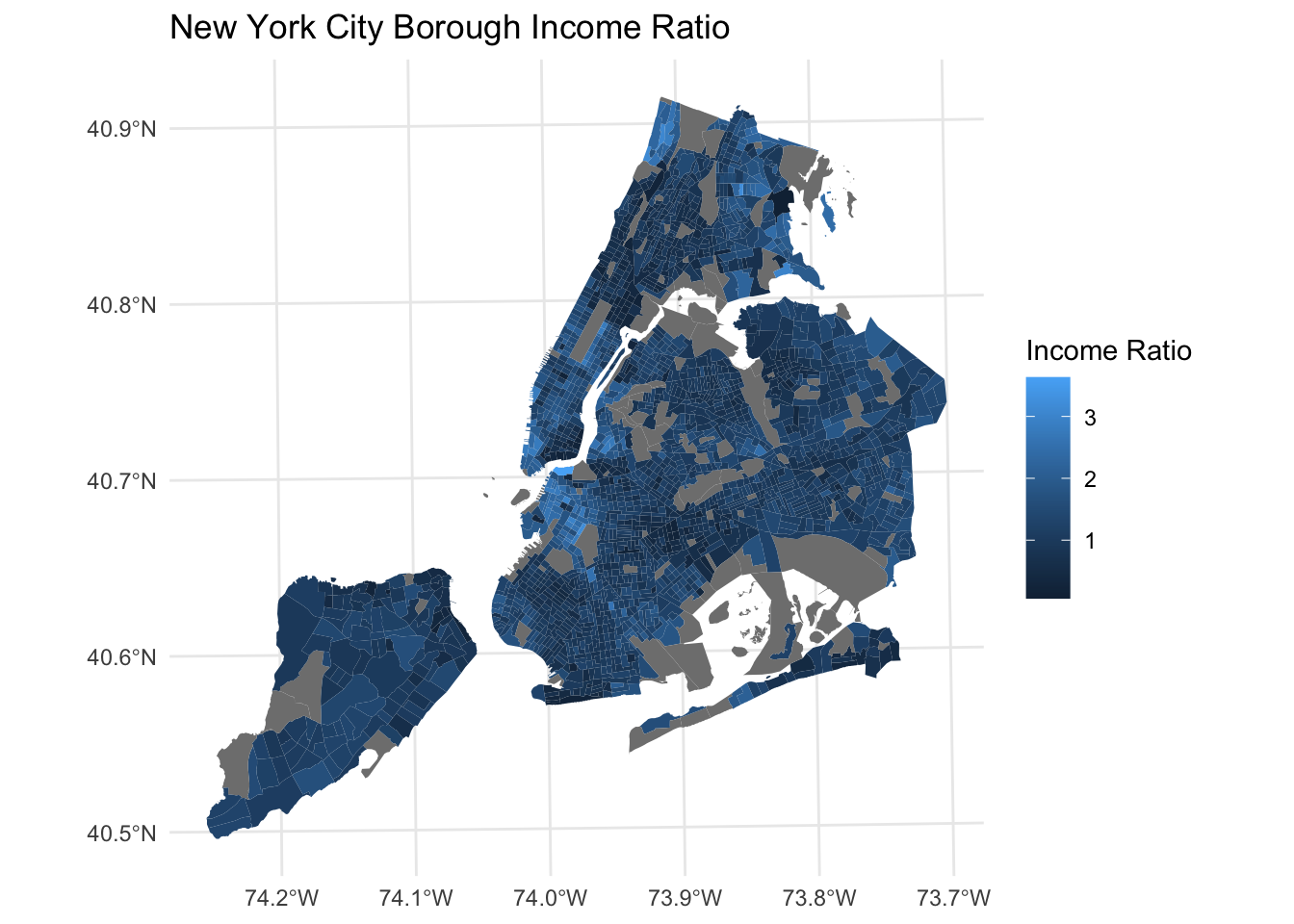

What would a ratio of 1 indicate? What would a ratio of 3 indicate? Where do we see big differences?

While we’re at it, it might be interesting to create a scatter plot that illustrates the relationship between racial concentration and income. To do this, we’ll need to join together our two datasets.

Code

nyc_dataset <- left_join(nyc_race, nyc_income |> st_set_geometry(NULL)|> select(GEOID, MHHIE, MHHIM, co_MHHIE, co_MHHIM, inc_ratio), by="GEOID")

Let’s plot the Percent White on the X axis and the income ratio on the y axis using geom_point):

Code

ggplot()+
  geom_point(data=nyc_dataset, aes(x=(WhiteE/PoptotE), y=inc_ratio), cex = .5, alpha = .2) +
  labs(title = "My Cool Plot", x = "Percent White", y = "Income Ratio") +
  scale_x_continuous(labels = scales::percent)+
  theme_minimal()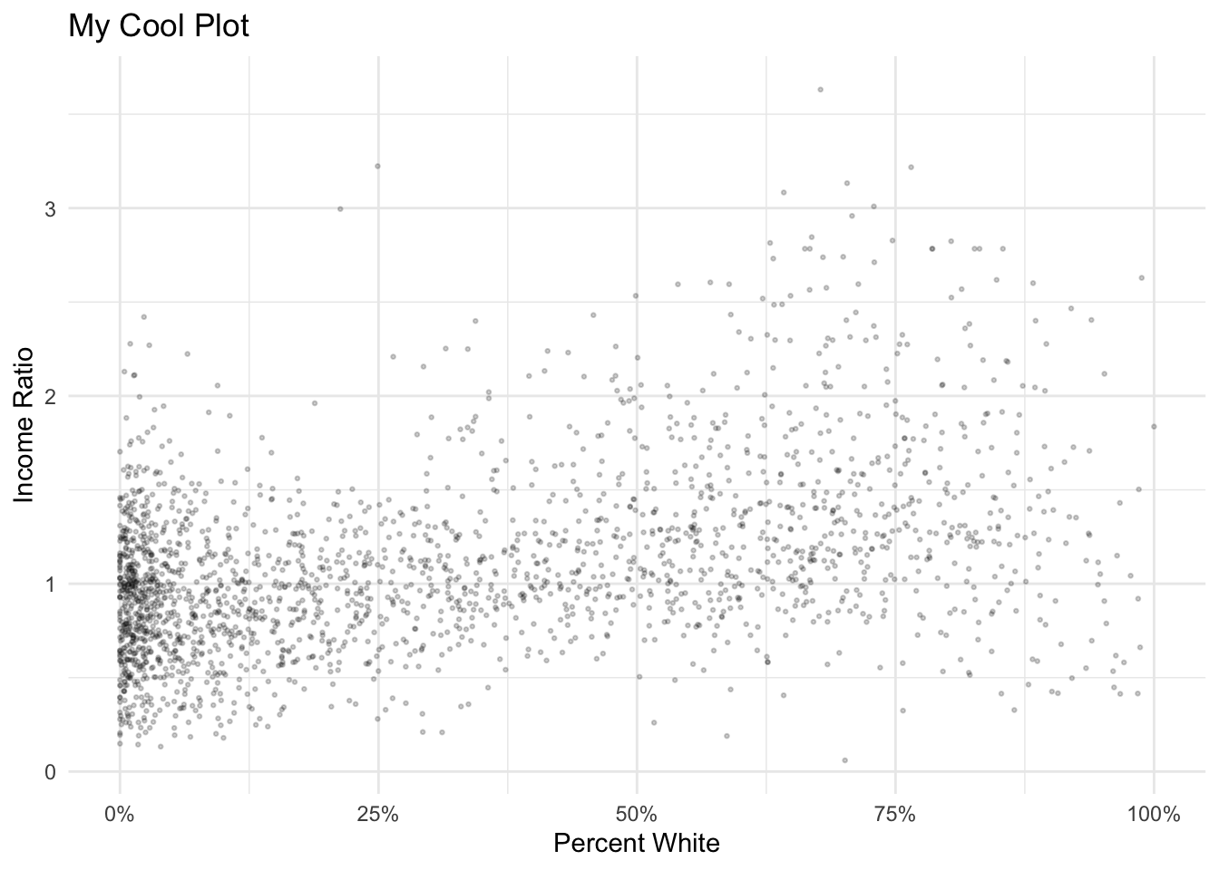

How would you describe this relationship?

Now see if you can add a linear line of best fit to these data using geom_smooth (you’ll need to set method = lm to get a fitted linear model):

Code

ggplot()+
  geom_point(data=nyc_dataset, aes(x=(WhiteE/PoptotE), y=inc_ratio), cex = .5, alpha = .2) +
  geom_smooth(data=nyc_dataset, method = "lm", aes(x=(WhiteE/PoptotE), y=inc_ratio), alpha = .5)+
  labs(title = "Tract Income Ratio by White Population", x = "Percent White", y = "Income Ratio") +
  scale_x_continuous(labels = scales::percent)+
  theme_minimal()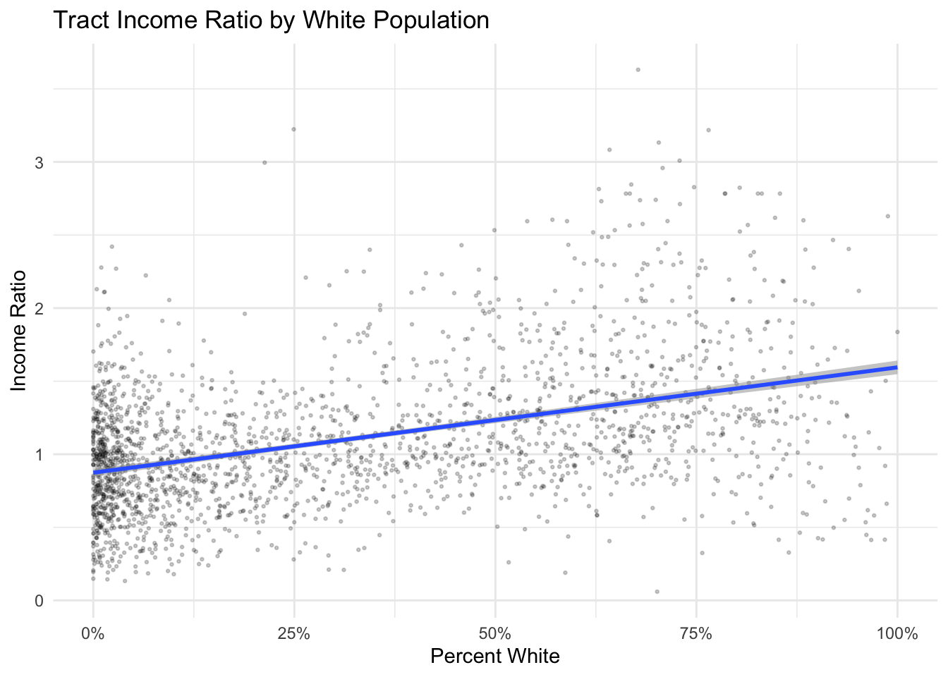

What’s the relationship between the percent white population and the income ratio?

What would it look like to split this out by boroughs using facets?

Code

ggplot()+
  geom_point(data=nyc_dataset, aes(x=(WhiteE/PoptotE), y=inc_ratio), cex = .5, alpha = .2) +
  geom_smooth(data=nyc_dataset, method = "lm", aes(x=(WhiteE/PoptotE), y=inc_ratio), alpha = .5)+
  labs(title = "Tract Income Ratio by White Population", x = "Percent White", y = "Income Ratio") +
  scale_x_continuous(labels = scales::percent)+
  theme_minimal()+
  facet_wrap(~Borough)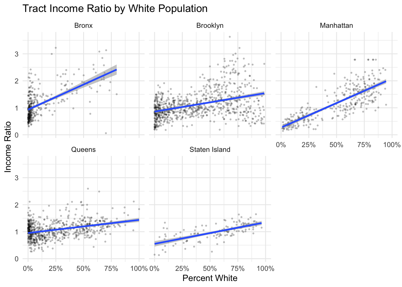

How would you describe the differences observed by boroughs?

Congratulations, you have learned some ways to calculate common measures of segregation, and have applied these measures as part of a data pipeline.

By changing your download calls at the very beginning of this lab where you download ACS data, you could easily create segregation measures for other places (note that you would have to re-label some elements where we indicate boroughs which are counties within New York City).

Extending this Analysis

Now that you have some new tools that you are familiar with, start exploring these data more. Make maps for other racial groups. Explore dimensions of segregation for other groups.

Can you produce the data which would populate a summary table of minority-majority dissimilarity? Which groups face the highest levels of segregation?
How does income relate to levels of segregation? Think about how you might use the median household income statistic to explore the relationship.
What are other forms of segregation that might be useful to explore (aside from racial and income segregation)?

Lab Evaluation

In evaluating your lab submission, we’ll be paying attention to the following:

Proper use of tigris tidycensus to download tabular and spatial data from the census bureau.
Production of clearly-labelled and well-formatted tables.
Production of well-formatted maps of income inequality.
Detailed reflection and diagnosis using measure of segregation.

As you get into the lab, please feel welcome to ask us questions, and please share where you’re struggling with us and with others in the class.

Introduction

Goals

Core Concepts

R and Rstudio

Github Lab Repository

Setup

Get Tract Boundaries

Get ACS Data

Create County Summaries

Setup Summary

Dissimilarity

Black-White Dissimilarity

Nonwhite-White Dissimilarity

Latino-White Dissimilarity

Interaction

Nonwhite-White Interaction

Latino-White Interaction

Isolation

Black Isolation

Nonwhite Isolation

Latino Isolation

Income Inequality

Extending this Analysis

Lab Evaluation

References