Segregation

Session Description

In this session, we will begin to work on a lab focused on measures of residential segregation. We will also spend some time workshopping your approach to the Population Memo.

We’ll take around 20 minutes at the beginning of class for you to share with each other what you’re thinking and your approach.

We’ll then engage any questions you have about this week’s lab or last week’s lab.

Before Class

Please come ready to share your approach to the population memo in small groups. Please bring in examples of analysis or visualization that we can look at, either in small groups or collectively.

Reflect

Code

In class, we spent some time looking at code that would select tracts within census place geographies. Here’s that code for your reference.

Let’s start by downloading tract and place geometries and selecting Chicago (as an example):

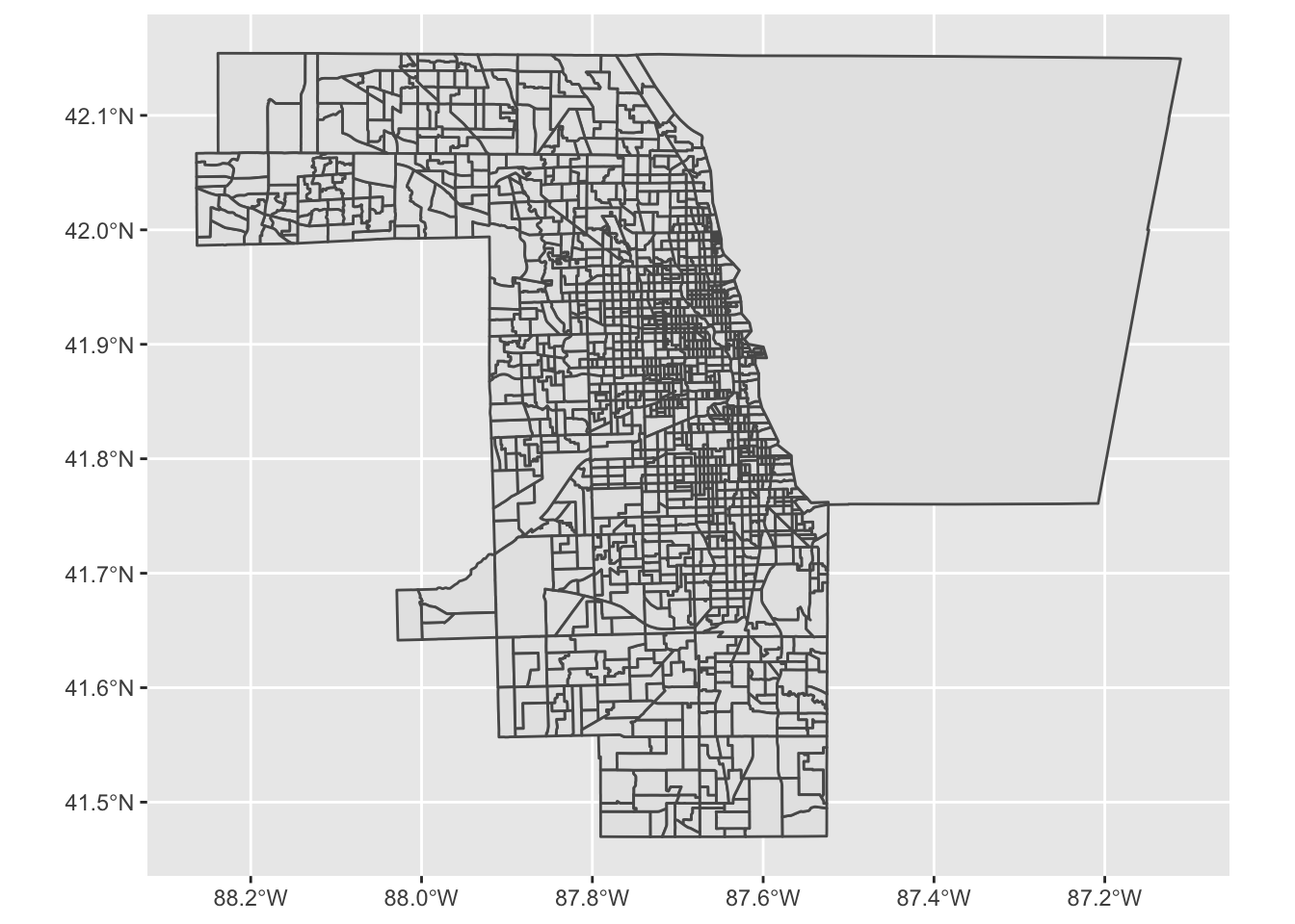
First, download tracts, subset to Cook County, and plot to confirm:

library(sf)
library(tigris)
library(tidyverse)


il_trt <- tracts(state = "IL") |> 
  filter(COUNTYFP == "031")


  |                                                                            
  |                                                                      |   0%
  |                                                                            
  |                                                                      |   1%
  |                                                                            
  |=                                                                     |   1%
  |                                                                            
  |=                                                                     |   2%
  |                                                                            
  |==                                                                    |   2%
  |                                                                            
  |==                                                                    |   3%
  |                                                                            
  |==                                                                    |   4%
  |                                                                            
  |===                                                                   |   4%
  |                                                                            
  |===                                                                   |   5%
  |                                                                            
  |====                                                                  |   5%
  |                                                                            
  |====                                                                  |   6%
  |                                                                            
  |=====                                                                 |   6%
  |                                                                            
  |=====                                                                 |   7%
  |                                                                            
  |=====                                                                 |   8%
  |                                                                            
  |=======                                                               |  10%
  |                                                                            
  |========                                                              |  11%
  |                                                                            
  |========                                                              |  12%
  |                                                                            
  |=========                                                             |  13%
  |                                                                            
  |==========                                                            |  14%
  |                                                                            
  |==========                                                            |  15%
  |                                                                            
  |===========                                                           |  15%
  |                                                                            
  |===========                                                           |  16%
  |                                                                            
  |============                                                          |  17%
  |                                                                            
  |============                                                          |  18%
  |                                                                            
  |=============                                                         |  19%
  |                                                                            
  |==============                                                        |  20%
  |                                                                            
  |===============                                                       |  22%
  |                                                                            
  |================                                                      |  22%
  |                                                                            
  |=================                                                     |  24%
  |                                                                            
  |=================                                                     |  25%
  |                                                                            
  |==================                                                    |  25%
  |                                                                            
  |==================                                                    |  26%
  |                                                                            
  |===================                                                   |  27%
  |                                                                            
  |====================                                                  |  28%
  |                                                                            
  |=====================                                                 |  30%
  |                                                                            
  |======================                                                |  31%
  |                                                                            
  |======================                                                |  32%
  |                                                                            
  |=======================                                               |  32%
  |                                                                            
  |========================                                              |  34%
  |                                                                            
  |=========================                                             |  36%
  |                                                                            
  |==========================                                            |  37%
  |                                                                            
  |===========================                                           |  38%
  |                                                                            
  |===========================                                           |  39%
  |                                                                            
  |============================                                          |  39%
  |                                                                            
  |============================                                          |  40%
  |                                                                            
  |=============================                                         |  41%
  |                                                                            
  |==============================                                        |  42%
  |                                                                            
  |==============================                                        |  43%
  |                                                                            
  |===============================                                       |  44%
  |                                                                            
  |===============================                                       |  45%
  |                                                                            
  |================================                                      |  45%
  |                                                                            
  |================================                                      |  46%
  |                                                                            
  |=================================                                     |  47%
  |                                                                            
  |=================================                                     |  48%
  |                                                                            
  |==================================                                    |  49%
  |                                                                            
  |===================================                                   |  50%
  |                                                                            
  |====================================                                  |  52%
  |                                                                            
  |=====================================                                 |  53%
  |                                                                            
  |======================================                                |  54%
  |                                                                            
  |======================================                                |  55%
  |                                                                            
  |=======================================                               |  55%
  |                                                                            
  |=======================================                               |  56%
  |                                                                            
  |========================================                              |  57%
  |                                                                            
  |========================================                              |  58%
  |                                                                            
  |=========================================                             |  59%
  |                                                                            
  |==========================================                            |  60%
  |                                                                            
  |===========================================                           |  61%
  |                                                                            
  |===========================================                           |  62%
  |                                                                            
  |============================================                          |  62%
  |                                                                            
  |============================================                          |  63%
  |                                                                            
  |============================================                          |  64%
  |                                                                            
  |=============================================                         |  64%
  |                                                                            
  |==============================================                        |  65%
  |                                                                            
  |==============================================                        |  66%
  |                                                                            
  |===============================================                       |  67%
  |                                                                            
  |===============================================                       |  68%
  |                                                                            
  |================================================                      |  68%
  |                                                                            
  |================================================                      |  69%
  |                                                                            
  |=================================================                     |  70%
  |                                                                            
  |===================================================                   |  72%
  |                                                                            
  |===================================================                   |  73%
  |                                                                            
  |====================================================                  |  74%
  |                                                                            
  |====================================================                  |  75%
  |                                                                            
  |=====================================================                 |  76%
  |                                                                            
  |======================================================                |  76%
  |                                                                            
  |======================================================                |  77%
  |                                                                            
  |=======================================================               |  78%
  |                                                                            
  |========================================================              |  79%
  |                                                                            
  |========================================================              |  80%
  |                                                                            
  |=========================================================             |  82%
  |                                                                            
  |==========================================================            |  82%
  |                                                                            
  |==========================================================            |  83%
  |                                                                            
  |============================================================          |  85%
  |                                                                            
  |============================================================          |  86%
  |                                                                            
  |=============================================================         |  87%
  |                                                                            
  |==============================================================        |  88%
  |                                                                            
  |==============================================================        |  89%
  |                                                                            
  |===============================================================       |  89%
  |                                                                            
  |================================================================      |  91%
  |                                                                            
  |=================================================================     |  93%
  |                                                                            
  |==================================================================    |  94%
  |                                                                            
  |==================================================================    |  95%
  |                                                                            
  |===================================================================   |  96%
  |                                                                            
  |====================================================================  |  97%
  |                                                                            
  |====================================================================  |  98%
  |                                                                            
  |===================================================================== |  98%
  |                                                                            
  |===================================================================== |  99%
  |                                                                            
  |======================================================================| 100%

ggplot()+
  geom_sf(data = il_trt)

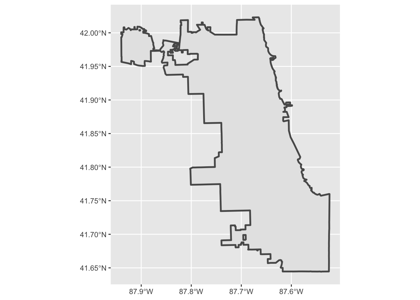
Next, download census place boundaries, filter to Chicago, and plot to confirm:

il_place <- places(state = "IL") |> 
  filter(NAME == "Chicago")


  |                                                                            
  |                                                                      |   0%
  |                                                                            
  |=                                                                     |   1%
  |                                                                            
  |=                                                                     |   2%
  |                                                                            
  |==                                                                    |   3%
  |                                                                            
  |=======                                                               |  10%
  |                                                                            
  |========                                                              |  12%
  |                                                                            
  |=========                                                             |  13%
  |                                                                            
  |==========                                                            |  14%
  |                                                                            
  |==========                                                            |  15%
  |                                                                            
  |===========                                                           |  16%
  |                                                                            
  |============                                                          |  17%
  |                                                                            
  |=============                                                         |  18%
  |                                                                            
  |=============                                                         |  19%
  |                                                                            
  |==============                                                        |  20%
  |                                                                            
  |==============                                                        |  21%
  |                                                                            
  |===============                                                       |  22%
  |                                                                            
  |================                                                      |  22%
  |                                                                            
  |================                                                      |  23%
  |                                                                            
  |=================                                                     |  24%
  |                                                                            
  |=================                                                     |  25%
  |                                                                            
  |==================                                                    |  26%
  |                                                                            
  |===================                                                   |  27%
  |                                                                            
  |====================                                                  |  28%
  |                                                                            
  |====================                                                  |  29%
  |                                                                            
  |=====================                                                 |  30%
  |                                                                            
  |======================                                                |  31%
  |                                                                            
  |======================                                                |  32%
  |                                                                            
  |=======================                                               |  33%
  |                                                                            
  |========================                                              |  34%
  |                                                                            
  |========================                                              |  35%
  |                                                                            
  |=========================                                             |  36%
  |                                                                            
  |==========================                                            |  37%
  |                                                                            
  |===========================                                           |  38%
  |                                                                            
  |===========================                                           |  39%
  |                                                                            
  |============================                                          |  40%
  |                                                                            
  |=============================                                         |  41%
  |                                                                            
  |=============================                                         |  42%
  |                                                                            
  |==============================                                        |  43%
  |                                                                            
  |===============================                                       |  44%
  |                                                                            
  |===============================                                       |  45%
  |                                                                            
  |================================                                      |  45%
  |                                                                            
  |================================                                      |  46%
  |                                                                            
  |=================================                                     |  47%
  |                                                                            
  |==================================                                    |  48%
  |                                                                            
  |===================================                                   |  50%
  |                                                                            
  |====================================                                  |  51%
  |                                                                            
  |=====================================                                 |  52%
  |                                                                            
  |=====================================                                 |  53%
  |                                                                            
  |======================================                                |  54%
  |                                                                            
  |======================================                                |  55%
  |                                                                            
  |=======================================                               |  56%
  |                                                                            
  |========================================                              |  58%
  |                                                                            
  |=========================================                             |  58%
  |                                                                            
  |=========================================                             |  59%
  |                                                                            
  |==========================================                            |  60%
  |                                                                            
  |==========================================                            |  61%
  |                                                                            
  |===========================================                           |  61%
  |                                                                            
  |===========================================                           |  62%
  |                                                                            
  |============================================                          |  62%
  |                                                                            
  |============================================                          |  63%
  |                                                                            
  |=============================================                         |  64%
  |                                                                            
  |==============================================                        |  65%
  |                                                                            
  |==============================================                        |  66%
  |                                                                            
  |===============================================                       |  67%
  |                                                                            
  |================================================                      |  68%
  |                                                                            
  |================================================                      |  69%
  |                                                                            
  |=================================================                     |  70%
  |                                                                            
  |==================================================                    |  71%
  |                                                                            
  |==================================================                    |  72%
  |                                                                            
  |===================================================                   |  73%
  |                                                                            
  |====================================================                  |  74%
  |                                                                            
  |=====================================================                 |  76%
  |                                                                            
  |======================================================                |  77%
  |                                                                            
  |=======================================================               |  78%
  |                                                                            
  |=======================================================               |  79%
  |                                                                            
  |========================================================              |  80%
  |                                                                            
  |=========================================================             |  81%
  |                                                                            
  |=========================================================             |  82%
  |                                                                            
  |==========================================================            |  83%
  |                                                                            
  |===========================================================           |  84%
  |                                                                            
  |===========================================================           |  85%
  |                                                                            
  |============================================================          |  85%
  |                                                                            
  |============================================================          |  86%
  |                                                                            
  |==============================================================        |  89%
  |                                                                            
  |===============================================================       |  90%
  |                                                                            
  |===============================================================       |  91%
  |                                                                            
  |================================================================      |  91%
  |                                                                            
  |=================================================================     |  92%
  |                                                                            
  |=================================================================     |  93%
  |                                                                            
  |==================================================================    |  94%
  |                                                                            
  |===================================================================   |  95%
  |                                                                            
  |===================================================================   |  96%
  |                                                                            
  |====================================================================  |  97%
  |                                                                            
  |====================================================================  |  98%
  |                                                                            
  |===================================================================== |  98%
  |                                                                            
  |===================================================================== |  99%
  |                                                                            
  |======================================================================| 100%

ggplot()+
  geom_sf(data = il_place, cex = 1)

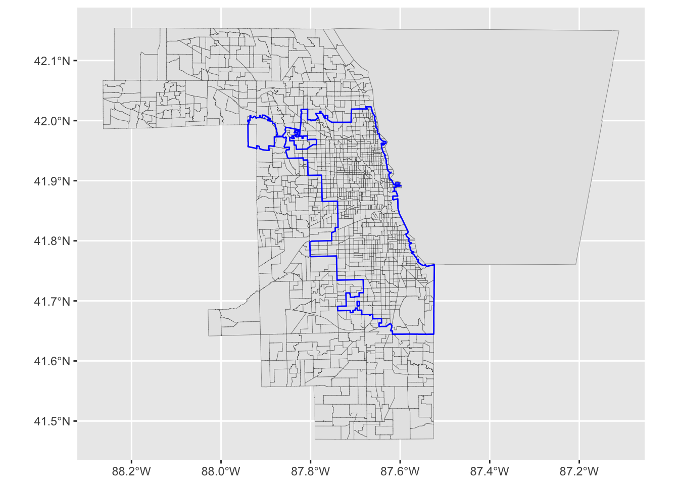
Plot together to see overlay:

ggplot()+
  geom_sf(data = il_trt, cex=.1)+
  geom_sf(data = il_place, color = "blue",cex = .5, fill = NA)

Option 1: Spatial Join

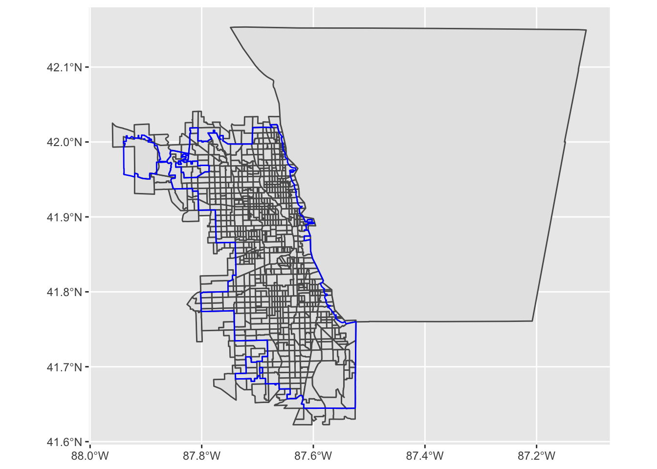
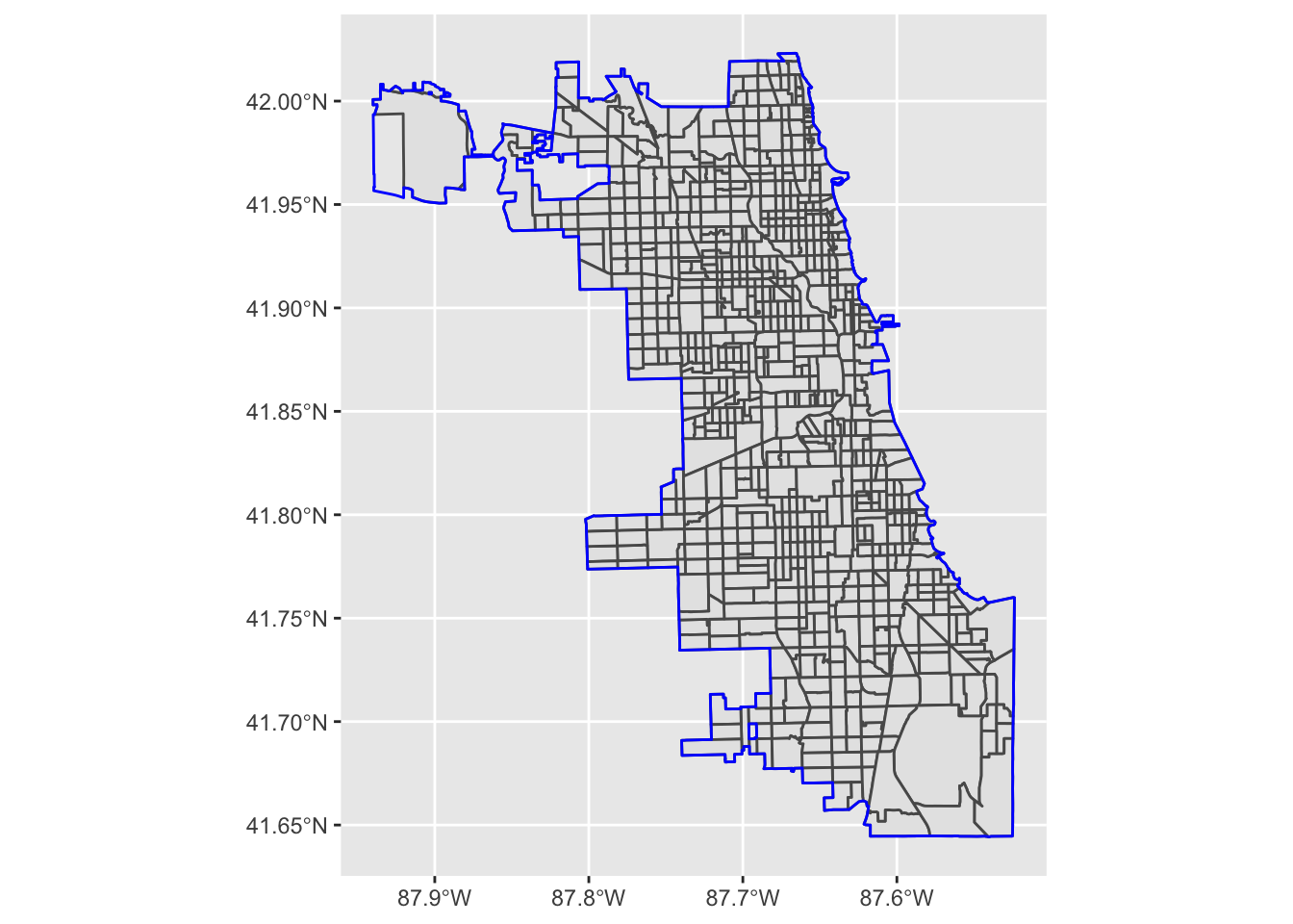
Perform a spatial join to identify all tracts that overlap with Chicago’s municipal boundaries, plot to confirm:

test <- st_join(il_trt, il_place) |> 
  filter(NAME.y == "Chicago")

ggplot() +
  geom_sf(data = test) +
  geom_sf(data = il_place, color = "blue", fill = NA)

Option 2: Intersection

Another option is to find the spatial intersection of the two objects:

test2 <- st_intersection(il_trt, il_place)

ggplot() +
  geom_sf(data = test2)+
  geom_sf(data = il_place, color = "blue", fill = NA)

As we discussed in class, there may be good reasons for pursuing either method. Intersection may produce visually “cleaner” output, but we may need to spend more time explaining that there are portions of tract geometry that fall outside of the city boundary. We may even want to do some analysis to estimate where uncertainty may come from due to our strategy.